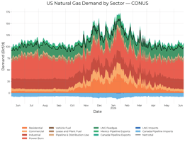
Our US Gas Demand release brought you daily demand estimates for today and the past. As promised,...
Our Full Supply & Demand Balances release makes forward supply and demand forecasts available alongside daily history and current estimates in hdl.gas_balance. This guide explains how to access the data, explore historical-weather scenarios, and use the table in your own analysis.
Overview demand information is already available on the SynMax front end, under Quickview.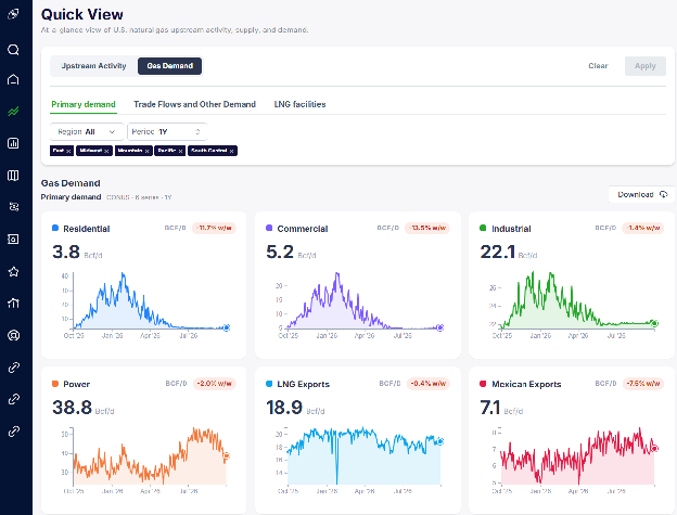
We are also building an extensive collection of pre-made demand and balance dashboards to make the forecasts, weather scenarios and common analytical workflows easier to explore without writing queries. Note that these use Agents on the backend, but they don’t consume your credit balances, nor do they require you to be authorized for Agents.
Explore the Gas Balances Quick Reference and pre-made dashboards
For custom analysis, use SynMax Agents. The data also remains accessible through the Hyperion v4 API's query_datalinks function for integration into your own workflows.
Use the Agent to Find Insight
What Does the Forward Balance Show?
“Show me the baseline CONUS supply and demand outlook for the next six months. Break out production, domestic consumption, trade and LNG feedgas, and show the implied monthly storage changes. Flag incomplete forecast periods.”
What If a Historical Weather Year Repeats?
“Replay 2014 weather for the coming winter and compare the resulting demand forecasts with the baseline. Show the differences by demand sector and EIA storage region, then quantify the effect on the complete national balance.”
How Wide Is the Weather-Driven Range?
“Compare the available historical-weather scenarios for the coming winter. Show the range of seasonal gas consumption and implied national storage changes, identify the years producing the highest and lowest demand, and highlight the ten-year demand baseline. Verify that each balance includes all required components.”
Which Sectors Drive the Differences?
“Compare next summer's baseline electric power demand with the individual historical-weather scenarios. Identify which regions contribute most to the variation and explain how the nonlinear cooling response affects the outlook.”
For API Users: The Next 30 Days
This starting query retrieves the baseline CONUS component forecasts for the next 30 gas days. It keeps the components separate so you can inspect the drivers before calculating the net balance. Note that bcf_day is signed - supply is positive, demand and exports negative.
SELECT date, component, bcf_day
FROM hdl.gas_balance
WHERE region = 'CONUS'
AND model_scenario = 'baseline'
AND weather_scenario = 'baseline'
AND date > CURRENT_DATE
AND date <= CURRENT_DATE + INTERVAL '30 days'
ORDER BY date, component;
Use this SQL through Agents or as the query supplied to query_datalinks. The bcf_day field is a signed daily rate in billion cubic feet per day. For historical-weather comparisons beyond the near-term forecast, select the relevant weather_scenario, such as analog_2014, and check its available dates and component coverage.
Understanding analog_XXXX
The weather_scenario field identifies the weather assumption behind a forecast. Values follow the format analog_XXXX, where XXXX is the historical weather year: for example, analog_2014 replays 2014 weather through the forward demand models. All demand components, even if they don’t have a weather relationship are included, to make querying easier. Note that we define these as gas years, so that winter of 2015-16 (Nov 1 to Mar 31) will be analog_2015. This means that if today you were to pull up the data for “analog_2015”, the data shown for Jan 5, 2027 will be the demand resulting from Jan 5, 2016’s data.
Use weather_scenario = 'baseline' for the continuous history and forecast series. Near-term demand uses the GFS weather forecast; historical-weather replay scenarios provide alternative demand outcomes beyond that horizon. Beyond the GFS horizon, the demand baseline is the average of the modeled outcomes from the most recent ten historical-weather years—currently analog_2016 through analog_2025. It averages ten demand-model results, not ten years of weather inputs. This preserves the modeled response to each year's cold spells and heat waves before averaging the resulting demand.
When building a continuous historical-weather comparison, retain the baseline for history and the near-term forecast, then use the chosen analog where available beyond the GFS horizon. Check the returned dates rather than assuming a fixed transition date. Keep model_scenario = 'baseline', compare each analog with the baseline separately, and verify component coverage before interpreting a scenario total as a complete national balance; do not assume every non-weather component has an analog-labeled row.
Important Query Rules
- Keep scenarios separate. Use
model_scenario = 'baseline'and select oneweather_scenarioat a time. Do not sum alternative weather scenarios together. - Use CONUS for complete balances. Regional production and consumption do not include the national-only trade, LNG and balancing-factor components. Never add CONUS totals to the five regions.
- Respect the signs. Supply is positive; demand and exports are negative. Sum the signed components directly for the net balance.
- Distinguish rates from volumes. Average daily rates for monthly Bcf/d comparisons. For storage change in Bcf, sum each day's net balance multiplied by one day over the period.
- Check coverage. Confirm all required components and dates are present before comparing scenarios or calculating seasonal storage changes.
Explore the forward supply and demand outlook
Table Reference: hdl.gas_balance
Datalink: Hyperion Production (1007). Row granularity: one gas day × region × component × model scenario × weather scenario. Units: signed Bcf/d. Refresh: intraday; updated_at records the last load for each point. Baseline history begins January 1, 2024, and continues into the forward forecast.
Detailed Schema
| Column | Type | Description and valid values |
|---|---|---|
date |
date |
Gas day represented by the row, for example 2026-01-15. Applies to historical estimates and forecast days alike. |
region |
text |
CONUS, East, Midwest, Mountain, Pacific, or South Central. Individual states are not included. Use CONUS for a complete national balance; regional coverage is limited to production and sectoral consumption. |
component |
text |
Supply, consumption, trade, LNG, or reconciliation category. The 14 component names and their geographic coverage are listed below. |
bcf_day |
double precision |
Signed daily volume in billion cubic feet per day: supply positive, demand and exports negative. Balancing Factor may be either sign. Sum signed components for a complete CONUS daily balance; average across dates for a period's average daily rate. |
model_scenario |
text |
Currently baseline; reserved for future forecast-model or assumption-set differentiation. Include this filter explicitly in queries. |
weather_scenario |
text |
baseline for the continuous history and forecast series; analog_2001 through analog_2025 identify historical-weather replay scenarios. Beyond the GFS horizon, the demand baseline averages the latest ten analog demand-model outcomes, currently 2016–2025. Check dates and component coverage for individual analogs. |
updated_at |
timestamptz |
Timestamp with time zone recording the point's last update, for example 2026-08-25 19:36:26.172699+00:00. This is the update time, not the gas day. Note that this is static for older values, one can query on this column to get only changed values. |
Component Values and Coverage
| Component | Sign | Geographic coverage |
|---|---|---|
Production |
Positive: supply | CONUS and all five EIA storage regions |
Canada Pipeline Imports |
Positive: supply | CONUS only |
LNG Imports |
Positive: supply | CONUS only |
Residential |
Negative: consumption | CONUS and all five EIA storage regions |
Commercial |
Negative: consumption | CONUS and all five EIA storage regions |
Industrial |
Negative: consumption | CONUS and all five EIA storage regions |
Electric Power |
Negative: consumption | CONUS and all five EIA storage regions |
Lease and Plant Fuel |
Negative: consumption | CONUS and all five EIA storage regions |
Pipeline & Distribution Use |
Negative: consumption | CONUS and all five EIA storage regions |
Vehicle Fuel |
Negative: consumption | CONUS and all five EIA storage regions |
LNG Feedgas |
Negative: gas delivered to LNG export terminals | CONUS only |
Canada Pipeline Exports |
Negative: exports | CONUS only |
Mexico Pipeline Exports |
Negative: exports | CONUS only |
Balancing Factor |
Positive or negative: reconciliation | CONUS only |
Production is already included in this table; no separate production-table join is needed to calculate the baseline national balance. Regional sums are not complete storage balances because trade, LNG and the balancing factor are available only at CONUS level.