Over the last few months we have observed deficiencies in how our legacy dry gas production model performed against EIA benchmarks. As a result we have updated this model to produce more granular monthly dry gas factors which can better account for volatile changes. The total change across the L48 is minimal for the most recent period with an impact of only -0.20 bcf/d for the most recent complete month of May 2025 when combined with this quarter's pipeline regression updates. However, the change is material in Texas and New Mexico with the two states' differences mostly offsetting between each other. We will be making this update live tomorrow 6/5 at the end of the day.
Note that these dry gas factor changes described below will also be applied at the same time as our quarterly regression modeling updates. The net difference to our current model is shown below. As you can see, though the change varies over time, the current value goes down by about 200 mmcf/d.


Because this is a completely new dry gas factor model the changes will retroactively impact the entire history of our daily production dataset up through today.
In this article we will break down exactly how our new dry gas factor model works, what new sources of data we are using to make our projections and the impact this has on our dry gas dataset at the sub-regional level.
Background
While our historic gross production matches EIA data, which is unsurprising given that EIA also sources their gross production from state production data, the story is different for our dry production.
Though our overall L48 production was very close, it was biased slightly high. (In all cases, error is computed as model minus “truth”, so that + error means we are high, and - error, low)


There are some states where there is a larger variance, seen below Our PA, WV, OH and GOM are near-perfect. ND has been good, but recently has started to deviate.

For these reasons, we looked for an improved approach to our dry gas modeling.
Analysis
We do not model dry production directly. Rather our current process calibrates summed pipeline scrapes by subregion to summed state production, to model gross withdrawals, then multiplies that value by a dry gas production factor. As you can see below, the implied state-level dry gas production factor for some states varies widely from other sources, leading to the conclusion that this model needs improvement. (We say implied, because we model by sub-region, but we took state totals to be able to compare to EIA and other sources.)


We had two choices to correct this:
- We can continue modeling wet and dry gas separately utilizing a more granular dry gas factor variable that tracks monthly changes.
- We can stop modeling dry gas factors altogether and instead model only dry gas separately from modeling wet gas, which would make the dry gas factors implied instead of explicit.
Correction 2 has one difficulty that makes it problematic:
- If we were to have two independent production models (gross and dry) then occasionally, our results might imply problematic or impossible dry gas production factors requiring explanation, which reduces model transparency.
Consequently, we have pursued option 1.
Correction 1 has its own modelling complexities that must be addressed.
- There is no source of “truth” for sub-state level dry production. We must make sure that our regional factors result in state-level values that are accurate.
Any model must result in a national-level dry gas production values that continue to be accurate
Our Solution
State-Level Approaches
For states that have only one sub-region per state, there is no difficulty, and little accuracy concerns. The dry gas factor for each state is easily determined from the EIA dry and gross production. However, the difficulty lies in states that have multiple subregions per state. There is no directly corresponding dry gas production at the subregion level.1
Our initial approach was to use optimization methods to attempt to determine the various sub-region factors that minimize the error in the overall state-level dry gas production. Unfortunately, there were one of two results: either the factors were unrealistic, given the known nature of a sub-region relative to others (for example, one model concluded Haynesville TX was far wetter than South TX), or we had to, a priori, restrict the ranges of the various regions, which substituted our judgement for the data.
For NM, several approaches were examined, and in all cases, the SJ basin ended up with very high factors, 0.98-0.99, and Permian moving to accommodate. We chose to just set SJ to 0.98 and adjust Permian to make zero error. This results in zero in-sample error.
For Colorado, we have San Juan and non-San Juan. Most NG processing in Colorado is NOT in the SJ basin, and we have the example of NM, so we’ve set the SJ basin to 0.98 and let the rest make up the dry gas. This results in zero error.
In the case of PA, we have two regions - NE PA, and SW PA. NE PA is truly dry gas, so we’ve just set NE PA to 0.995 and let SWPA dry gas factor be whatever it takes to get to the state totals. This also results in zero error.
In the case of LA, the overall average dry gas factor is so high (between 0.99 and 1.02, since due to LA offshore reporting issues you can actually have a factor > 1), and given the domination of Haynesville in LA production, the only approach that gives reasonable results is to set all regions to the overall LA average dry gas factor. This results in zero error in-sample.
For TX, the RRC has a report with aggregate extraction by RRC district https://www.rrc.texas.gov/oil-and-gas/research-and-statistics/production-data/monthly-summary-of-texas-natural-gas/ The value in this is that it allows us to make sure that the various sub-regions have the appropriate relationship to each other in developing the state-wide numbers. Though it has overall extraction loss for the entire state, the valuable data is the per-district NGL production. Our first approach was to attempt to directly convert barrels of ngl production into extraction loss, but the unreported physical properties and aggregations made this process very difficult, and yielded unrealistic results.
We turned to statistical methods. Since we only have dry gas fractions for the entire state, we can only examine the relationship at a state level. We develop a liquids ratio in bbl/mcf as:
LiqRatioi = Total Liquidsi - Lease Condensatei_________
Transmissions Linesi + Processing Plantsi
Where i is for each RRC district and for the whole state, with liquids data from Table 6 and gas data from tables 4 and 5 in the Texas state summary.
There is clearly a relationship, as seen below (the upper-left point is a “fake” point, but one that is a very real physical constraint - at 0 bbls NGL production, the dry gas fraction is 1.0). The difficulty here is that we only have dry gas data for the entire state, and some districts have extraction amounts in excess of the range of values in the state-wide data. That means that our model for converting the liquids ratio must use the state-wide totals, then we assume that the relationship should hold for each district.

The linear model has issues at the dryer levels. The Polynomial model performs well at the dryer levels, but the curve at the wetter levels is completely unsuitable. The Exponential performance is pretty good, but flattens out at approximately 0.77 dry gas factor, which is unacceptable, since some districts have much higher liquids ratios and therefore must have lower dry gas factors. So, we are going to patch the exponential and linear models - above 0.058 liquids ratio, we use linear, and below, exponential, with the following resulting model. The resultant model fits with a r2 of about 0.82.
However, this results in a slight error in total overall forecast dry gas volume.

To solve this we use a rolling linear regression model to adjust the factors, with the following graphs showing the resulting factors, and the resultant error. (NB, the adjustment never exceeds 2%).


Overall Result
Note that the regression update only changes production for dates more recent than the last good dates for each state’s data, so that error calculations against EIA dry data, which ends in 2023, are purely a result of dry gas factor changes.
The resultant L48 error is overall the same with the mean squared error essentially identical (better, but by < 0.5% difference).

Those with multiple SRs show substantial improvement:

And the other states error:

Finally all dry gas factors are projected forward from their end data (usually end of 2023) to 18 months after the calibration date, by:
- The first forward month is set to the average of the last 6 months.
- The factor initially moves at the same trend as the last 24 months average trend (average determined by simple linear regression).
- The rate of change of the factor decays to 0 in 18 months.
- The factor is kept constant after this.
Conclusion
We believe that this improvement in our dry gas factor model allows us to better explain the changing differences between wet and dry gas production directly instead of relying on implied factors like others do. In essence we have decided to maintain two separate models. Wet gas production forecasting and dry gas factor forecasting, the combination of these two models gives us our dry gas numbers with greater control and better explainability. It is also a much better base model structure for later planned additions to our datasets including propane, ethane and butane production forecasting.
The dry gas factor model results, including our factor forecasts can now be queried from our API, python client and Snowflake tables with plans to add this to our next Excel add-in release.
Here is an example of how to access them using our Python Library (be sure you have at least version 4.4.0 of the python package)
import osfrom synmax.hyperion import v4
access_token=os.environ.get("ACCESS_TOKEN")v4client = v4.HyperionApiClient(access_token)for item in v4client.dry_gas_factors(): print(item)
For any questions about this model change please reach out to us directly support@synmax.com.
Endnotes
- For TX, NM, and LA, there is some additional EIA data that theoretically could have been useful. The EIA “Dry shale gas production estimates by play” (now part of the EIA’s monthly report, called the Short Term Energy Outlook, STEO) has data for many “plays” in the US. This makes it very difficult to use, for example, the “Marcellus” and “Utica” data, since the state production data makes it very difficult to distinguish the source formation for production (in many cases the data is present, but would take extensive and dubious modelling to extract.)
-3.png?height=200&name=image%20(1)-3.png)