
Power burn, the gas burned to generate electricity, is the largest single use of US natural gas, and over the next two years it will be moved by things its history does not contain: data centers connecting to the grid, a wave of new solar and wind, and a diminished coal fleet competing with gas at forward prices. A trend fitted to EIA's record cannot see any of them, so our long-term forecast builds burn from those drivers instead, region by region and day by day. Where the utilities' load forecasts lean on data centers, we check them against what Vulcan, SynMax's satellite tracking of power projects, sees actually being built.
This note goes one level deeper than Inside the SynMax Electric Power Long-Term Forecast into how each piece is modeled: the generation components first, then the gas ceiling they add up to, the gas-versus-coal model on top, and finally how the method does when re-run from past dates.
How the Forecast Is Built
The forecast covers the five EIA gas storage regions (East, Midwest, South Central, Mountain, and Pacific), daily, two years ahead, with one path for each historical weather year. It works in three steps.
First, we forecast how much electricity each region will need, and how much of it nuclear, hydro, wind, solar, storage, and other sources will supply. What is left has to come from fossil-fuelled plants, which we call thermal generation. Second, we convert that thermal generation into gas at the fleet's heat rate. The result, the gas ceiling, is the most gas the region could burn if every thermal megawatt-hour came from gas. Third, a daily model sets how much of that ceiling gas actually captures from coal. The forecast is the ceiling times gas's share.
Electricity Demand and Load Growth
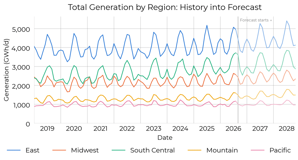
Total generation is the electricity a region needs. Its growth comes from the load forecasts the region's utilities file with FERC, plus ERCOT's for Texas. The filings also give the new load's shape: a data center draws about the same power in April as in August, so where filed summer peaks grow more slowly than filed energy, the added load is flatter than today's. The year's added energy is the same either way; only its spread through the year changes.
That growth starts from today's level with weather taken out. We fit EIA's plant-level generation (EIA-923) for each region's states against the time of year and heating and cooling demand, and remove both from the last twelve months, so a hot summer is not mistaken for growth.
Adjusting the Filings with Vulcan
The filings are the input that needs the most judgement. Our analysts adjust them, informed by Vulcan's satellite tracking of about 2,700 US data-center sites. Vulcan records when land is cleared, when structures go up, and when construction finishes, which splits each region's data-center pipeline into capacity operating, under construction, and announced only. Growth that leans on announced load with nothing built is cut; where the new load is data centers already under construction, more of it is treated as round-the-clock.
Other Generating Sources
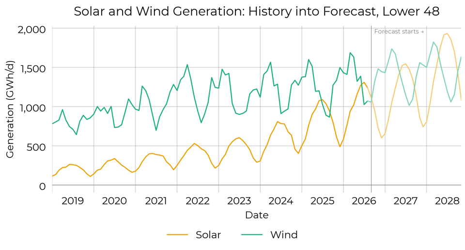
Wind and solar are each forecast as installed capacity times capacity factor. Capacity is today's operating fleet, from EIA's monthly generator inventory (EIA-860M), plus announced projects. Each project is discounted by how often similar projects have arrived on schedule, again informed by Vulcan observations.The capacity factor for each time of year is the average of the last three years of EIA data. Three years did best in backtests: long enough to average out an unusually still or cloudy year, short enough to follow capacity factors that are shifting as the fleet changes. A capacity factor one percentage point higher across the Lower 48 fleet would lower gas burn by about 0.28 Bcf/d for solar and 0.22 Bcf/d for wind. We are working on adding solar irradiance and wind speed data, so that wind and solar output follows each year's weather, which will improve upon our capacity factor.
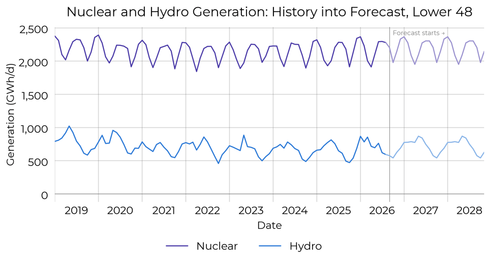
Nuclear and hydro follow their typical seasonality from the last ten years. For nuclear, that pattern carries the spring and fall refueling outages; for hydro, the spring runoff and late-summer decline of a typical water year.
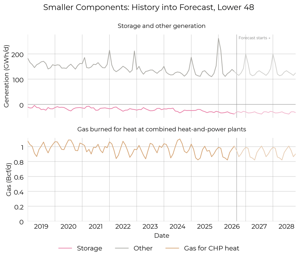
The smaller pieces follow their recent seasonality: storage (batteries and pumped hydro), other generation, including oil, and the gas that combined heat-and-power (CHP) plants burn for heat rather than electricity.
The Gas Ceiling
Subtracting those sources from total generation leaves thermal generation. Multiplying it by the fleet's heat rate, the gas burned per megawatt-hour of gas-fired generation over the last year with its usual seasonal shape, and adding the gas burned for combined heat and power gives the gas ceiling. It is built day by day: total generation follows each day's weather and the grid's weekday and holiday pattern, and the other pieces are spread smoothly within each month.
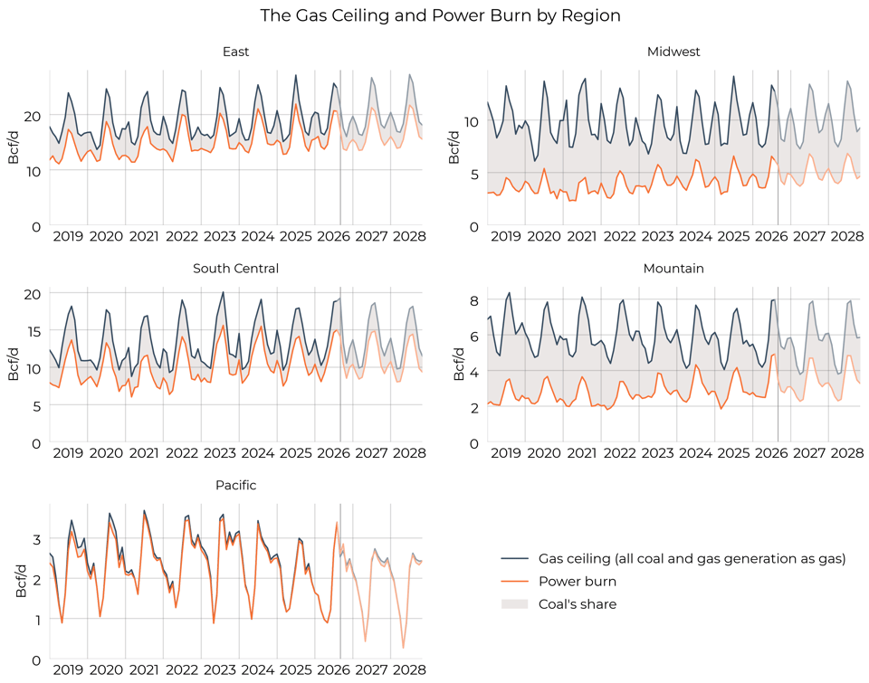
In the chart below, the gap between the ceiling and actual burn is the generation coal supplies, plus a little oil.
Gas Versus Coal
The last step decides how much of the ceiling gas captures. A model of daily power burn (our EIA-calibrated nowcast) divided by the gas ceiling explains gas's share, region by region, from three things: seasonal heating and cooling demand; the day of the week and holidays; and the share of thermal capacity where coal is cheaper than gas. The Pacific, with almost no coal, uses only the first two.
Where coal is cheaper is worked out plant by plant: the cost of a megawatt-hour from each coal plant is compared with the cost from gas in the same market, with coal priced on EIA's Short-Term Energy Outlook path and gas on the Henry Hub forward curve plus local basis. The coal fleet, including announced retirements, comes from EIA-860M. Prices are read at every run, so a move in the curve passes straight into the forecast; that is also the only way the gas price reaches burn, which is what the article's sensitivity chart shows when it shifts the curve $1/MMBtu up and down.
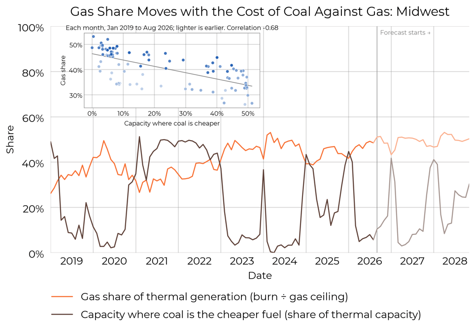
Most Midwest coal plants cost $20–35/MWh to run, so when gas crosses that range most of the fleet flips at once. That is why the share of capacity where coal is cheaper jumps between near zero and half.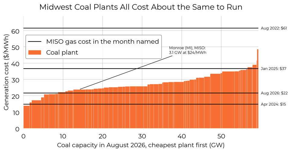
Weather Years
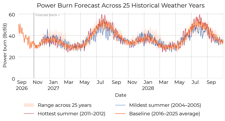
For the first two weeks every region runs on the latest NOAA ensemble weather forecast, which then fades into the day-by-day weather of each historical year from 2001 through 2025, one path each. The baseline is the average of the ten most recent paths: an average of demand outcomes, not demand at average weather.
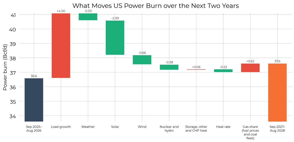
The Two-Year Driver Breakdown
The chart below compares the last twelve months of EIA data, September 2025 to August 2026, with the forecast's second year, September 2027 to August 2028, region by region. The bars add up exactly to the change, with nothing left over. The weather bar is the models' estimate of how much burn changes because last year's weather differed from the ten-year average the baseline is built on.
Performance
We re-ran the whole method as of March 31 of 2024, 2025, and 2026, refitting every model on only what was known on each date: EIA's plant data, the generator inventory, the coal fleet and fuel prices, and the utilities' filings as they then stood, with no analyst adjustments. Each run is handed the weather that actually happened, so the test measures the model rather than the weather call. Each date is run twice: once on the filings of the time, and once given the electricity demand EIA later reported, which makes the load call exact and isolates the rest of the model. Both are scored month by month against our EIA-calibrated daily power burn, summed over the five regions.
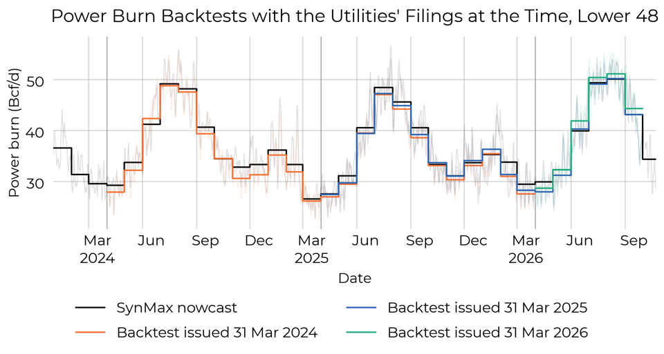
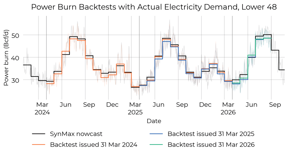
The table gives the monthly misses for the Lower 48: the backtest minus measured burn, positive where the backtest ran above. The typical miss is the root mean square.
| Issued | Load | Months scored | Mean miss (Bcf/d) | Typical miss (Bcf/d) | Mean absolute miss |
|---|---|---|---|---|---|
| March 31, 2024 | Filings at the time | 24 | −1.05 | 1.36 | 3.3% |
| March 31, 2025 | Filings at the time | 18 | −0.58 | 1.07 | 2.4% |
| March 31, 2026 | Filings at the time | 6 | +0.66 | 1.21 | 2.7% |
| March 31, 2024 | Actual demand | 24 | −0.35 | 1.01 | 2.3% |
| March 31, 2025 | Actual demand | 17 | −0.84 | 1.32 | 3.2% |
| March 31, 2026 | Actual demand | 5 | −0.98 | 1.41 | 3.6% |
On this year's filings the 2026 run is high, putting July to September 2026 at 48.6 Bcf/d against 47.6 Bcf/d measured. Given the demand that actually occurred, the same run is low over July and August, at 48.3 against 49.7, so the excess comes from this year's filings. That is why we check them against what Vulcan sees being built.
Data sources: EIA-923 plant-level generation and fuel consumption; EIA-860M monthly generator inventory; FERC Form 714 utility load forecasts; ERCOT Long-Term Load Forecast; Vulcan satellite-verified power project and data-center tracking; NOAA GEFS ensemble weather forecasts; the Henry Hub forward curve and regional basis; EIA Short-Term Energy Outlook coal price path.